
Advertisements
Advertisements
For the company A:
We know, based on our answer in Exercise 1.4, that the sample mean for samples in Company A is 
To compute for the sample variance, we shall use the formula
The formula states that we need to get the sum of 
Note: You can refer to the solution of Exercise 1.7 on how to use a table to solve for the variance.
The variance is
The standard deviation is just the square root of the variance. That is
For Company B:
Using the same method employed for Company A, we can show that the variance and standard deviation for the samples in Company B are


According to the journal Chemical Engineering, an important property of a fiber is its water absorbency. A random sample of 20 pieces of cotton fiber is taken and the absorbency on each piece was measured. The following are the absorbency values:
| 18.71 | 21.41 | 20.72 | 21.81 | 19.29 | 22.43 | 20.17 |
| 23.71 | 19.44 | 20.50 | 18.92 | 20.33 | 23.00 | 22.85 |
| 19.25 | 21.77 | 22.11 | 19.77 | 18.04 | 21.12 |
a. Calculate the sample mean and median for the above sample values.
b. Compute the 10% trimmed mean.
c. Do a dot plot of the absorbency data.
Since the champion plays better than the father, it seems reasonable that fewer sets should be played with the champion. On the other hand, the middle set is the key one, because Elmer cannot have two wins in a row without winning the middle one. Let C stand for the champion, F for father, and W and L for win and loss by Elmer. Let f be the probability of Elmer’s winning any set from his father, c the corresponding probability of winning from the champion. The table shows only possible prize-winning sequences together with their probabilities, given independence between sets, for the two choices.
Set with:
Father First
| F | C | F | Probability |
| W | W | W | fcf |
| W | W | L | fc(1-f) |
| L | W | W | (1-f)cf |
| Total | fc(2-f) |
Champion First
| C | F | C | Probability |
| W | W | W | cfc |
| W | W | L | cf(1-c) |
| L | W | W | (1-c)fc |
| Total | fc(2-c) |
Since Elmer is more likely to best his father than to beat the champion, f is larger than c, and 2-f is smaller than 2-c, and so Elmer should choose CFC. For example, for f=0.8, c=0.4, the chance of winning the prize with FCF is 0.384, that for CFC is 0.512. Thus, the importance of winning the middle game outweighs the disadvantage of playing the champion twice.
Many of us have a tendency to suppose that the higher the expected number of successes, the higher the probability of winning a prize, and often this supposition is useful. But occasionally a problem has special conditions that destroy this reasoning by analogy. In our problem, the expected number of wins under CFC is 2c+f, which is less than the expected number of wins for FCF, 2f+c. In our example with f=0.8 and c=0.4, these means are 1.6 and 2.0 in that order. This opposition of answers gives the problem flavor.
Just to set the pattern, let us do a numerical example first. Suppose there were 5 red and 2 black socks; then the probability of the first sock’s being red would be 5/(5+2). If the first were red, the probability of the second’s being red would be 4/(4+2), because one red sock has already been removed. The product of these two numbers is the probability that both socks are red:
\frac{5}{5+2}\times \frac{4}{4+2}=\frac{5\left( 4 \right)}{7\left( 6 \right)}=\frac{10}{21}This result is close to 1/2, but we need exactly 1/2. Now let us go at the problem algebraically.
Let there be r red and b black socks. The probability of the first sock’s being red is \frac{r}{r+b}; and if the first sock is red, the probability of the second’s being red now that a red has been removed is \frac{r-1}{r+b-1}. Then we require the probability that both are red to be \frac{1}{2}, or
\frac{r}{r+b}\times \frac{\:r-1}{r+b-1}=\frac{1}{2}One could just start with b=1 and try successive values of r, then go to b=2 and try again, and so on. That would get the answer quickly. Or we could play along with a little more mathematics. Notice that
\frac{r}{r+b}>\frac{\:r-1}{r+b-1}Therefore, we can create the inequalities
\left(\frac{r}{r+b}\right)^2>\frac{1}{2}>\left(\frac{\:r-1}{r+b-1}\right)^2Taking the square roots, we have, for r>1.
\frac{r}{r+b}>\frac{1}{\sqrt{2}}>\frac{\:r-1}{r+b-1}From the first inequality we get
r>\frac{1}{\sqrt{2}}\left( r+b \right)or
\begin{align*}
r & >\frac{1}{\sqrt{2}-1}b \\ \\
r & > \left( \sqrt{2}+1 \right)b
\end{align*}
From the second we get
\left( \sqrt{2}+1 \right)b>r-1or all told
\left(\sqrt{2}+1\right)b+1>r>\left(\sqrt{2}+1\right)bFor b=1, r must be greater than 2.414 and less than 3.414, and so the candidate is r=3. For r=3, \ b=1, we get
P\left(2\:\text{red socks}\right)=\frac{3}{4}\cdot \frac{2}{3}=\frac{1}{2}And so, the smallest number of socks is 4.
Beyond this, we investigate even values of b.
| b | r is between | eligible r | P\left(2 \ \text{red socks}\right) |
| 2 | 5.8, 4.8 | 5 | \frac{5\left( 4 \right)}{7\left( 6 \right)} \neq \frac{1}{2} |
| 4 | 10.7, 9.7 | 10 | \frac{10\left( 9 \right)}{14\left( 13 \right)} \neq \frac{1}{2} |
| 6 | 15.5, 14.5 | 15 | \frac{15\left( 14 \right)}{21\left( 20 \right)} = \frac{1}{2} |
And so, 21 is the smallest number of socks when b is even. If we were to go on and ask for further values of r and b so that the probability of two red socks is 1/2, we would be wise to appreciate that this is a problem in the theory of numbers. It happens to lead to a famous result in Diophantine Analysis obtained from Pell’s equation. Try r = 85, b = 35.
Questions:
Continue reading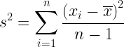


You must be logged in to post a comment.